tarprof

We create the targets pipeline as normal:

targets::tar_script({
  list(
    tar_target(sizes, c(10E6, 10E7, 10E8)),
    tar_target(make_vectors, numeric(sizes), pattern = map(sizes))
  )
}, ask = FALSE)

We need to specify a directory that will be used to save the profiling results:

monitor_path <- file.path(getwd(), "profile_results")

When it comes to running, we pass in the custom callr_function. In addition, we need to pass that function arguments using callr_arguments. One of these arguments must be monitor_path.

targets::tar_make(
  callr_function = tarprof::callr_profile,
  callr_arguments = list(
    monitor_path = monitor_path
  )
)

Note that for the moment, it is not recommended that you use any parallelism when running the pipeline in profiling mode. In other words, when calling crew::crew_controller_local, use workers = 1. Eventually I hope to lift this limitation.

Once the targets pipeline has finished, we can access the profiling data using tarprof::profile_data. This returns a data frame where each row is one timepoint, and the columns correspond to various process metrics.

profile <- tarprof::profile_data(monitor_path)
profile

## # A tibble: 371 × 16
##          rss       vms shared  text   lib   data dirty    uss    pss  swap  user
##        <dbl>     <dbl>  <dbl> <dbl> <dbl>  <dbl> <dbl>  <dbl>  <dbl> <dbl> <dbl>
##  1 124297216    3.43e8 7.58e6  4096     0 1.88e8     0 1.17e8 1.19e8     0  1.02
##  2 129732608    3.48e8 7.81e6  4096     0 1.93e8     0 1.23e8 1.24e8     0  1.13
##  3 209747968    4.28e8 7.81e6  4096     0 2.73e8     0 2.03e8 2.04e8     0  1.21
##  4 209747968    4.28e8 7.81e6  4096     0 2.73e8     0 2.03e8 2.04e8     0  1.32
##  5 209747968    4.28e8 7.81e6  4096     0 2.73e8     0 2.03e8 2.04e8     0  1.43
##  6 209747968    4.28e8 7.81e6  4096     0 2.73e8     0 2.03e8 2.04e8     0  1.54
##  7 209747968    4.28e8 7.81e6  4096     0 2.73e8     0 2.03e8 2.04e8     0  1.65
##  8 209797120    4.28e8 7.81e6  4096     0 2.73e8     0 2.03e8 2.04e8     0  1.76
##  9 292786176    1.23e9 7.81e6  4096     0 1.07e9     0 3.03e8 3.04e8     0  1.84
## 10 606646272    1.23e9 7.81e6  4096     0 1.07e9     0 6.18e8 6.19e8     0  1.85
## # ℹ 361 more rows
## # ℹ 5 more variables: system <dbl>, children_user <dbl>, children_system <dbl>,
## #   time <dttm>, pid <int>

However, this information isn’t much help without the knowledge of which targets were run at which times. We can integrate this information using tarprof::profile_per_target:

per_target <- tarprof::profile_per_target(profile)
per_target

## # A tibble: 16 × 40
##       rss    vms shared  text   lib data_profile dirty    uss    pss  swap  user
##     <dbl>  <dbl>  <dbl> <dbl> <dbl>        <dbl> <dbl>  <dbl>  <dbl> <dbl> <dbl>
##  1 2.10e8 4.28e8 7.81e6  4096     0    273293312     0 2.03e8 2.04e8     0  1.65
##  2 1.01e9 1.23e9 7.81e6  4096     0   1073295360     0 1.00e9 1.00e9     0  7.22
##  3 1.01e9 1.23e9 7.81e6  4096     0   1073295360     0 1.00e9 1.00e9     0  7.34
##  4 1.01e9 1.23e9 7.81e6  4096     0   1073295360     0 1.00e9 1.00e9     0  7.47
##  5 9.01e9 9.23e9 7.81e6  4096     0   9073299456     0 9.00e9 9.00e9     0 68.7 
##  6 9.01e9 9.23e9 7.81e6  4096     0   9073299456     0 9.00e9 9.00e9     0 68.9 
##  7 9.01e9 9.23e9 7.81e6  4096     0   9073299456     0 9.00e9 9.00e9     0 69.2 
##  8 9.01e9 9.23e9 7.81e6  4096     0   9073299456     0 9.00e9 9.00e9     0 69.4 
##  9 9.01e9 9.23e9 7.81e6  4096     0   9073299456     0 9.00e9 9.00e9     0 69.6 
## 10 9.01e9 9.23e9 7.81e6  4096     0   9073299456     0 9.00e9 9.00e9     0 69.8 
## 11 9.01e9 9.23e9 7.81e6  4096     0   9073299456     0 9.00e9 9.00e9     0 70.1 
## 12 9.01e9 9.23e9 7.81e6  4096     0   9073299456     0 9.00e9 9.00e9     0 70.3 
## 13 9.01e9 9.23e9 7.81e6  4096     0   9073299456     0 9.00e9 9.00e9     0 70.5 
## 14 9.01e9 9.23e9 7.81e6  4096     0   9073299456     0 9.00e9 9.00e9     0 70.7 
## 15 9.01e9 9.23e9 7.81e6  4096     0   9073299456     0 9.00e9 9.00e9     0 70.9 
## 16 9.01e9 9.23e9 7.81e6  4096     0   9073299456     0 9.00e9 9.00e9     0 71.2 
## # ℹ 29 more variables: system <dbl>, children_user <dbl>,
## #   children_system <dbl>, time_profile <dttm>, pid <int>, name <chr>,
## #   type <chr>, data_targets <chr>, command <chr>, depend <chr>, seed <int>,
## #   path <list>, time_targets <dttm>, size <chr>, bytes <dbl>, format <chr>,
## #   repository <chr>, iteration <chr>, parent <chr>, children <list>,
## #   seconds <dbl>, warnings <chr>, error <chr>, end_time <dttm>,
## #   start_time <dttm>, mid_time <dttm>, preceding_end <dttm>, …

Next, we can use the built-in summary function to get the maximum memory usage and CPU efficiency of each target:

profile_summary <- tarprof::summarise_targets(per_target)
profile_summary

## # A tibble: 3 × 4
##   name                          peak_memory peak_memory_time    cpu_efficiency
##   <chr>                               <dbl> <dttm>                       <dbl>
## 1 make_vectors_207c35afd65876c8   209747968 2024-05-29 12:00:19          0    
## 2 make_vectors_9105835678f0321b  1009717248 2024-05-29 12:00:25          0.653
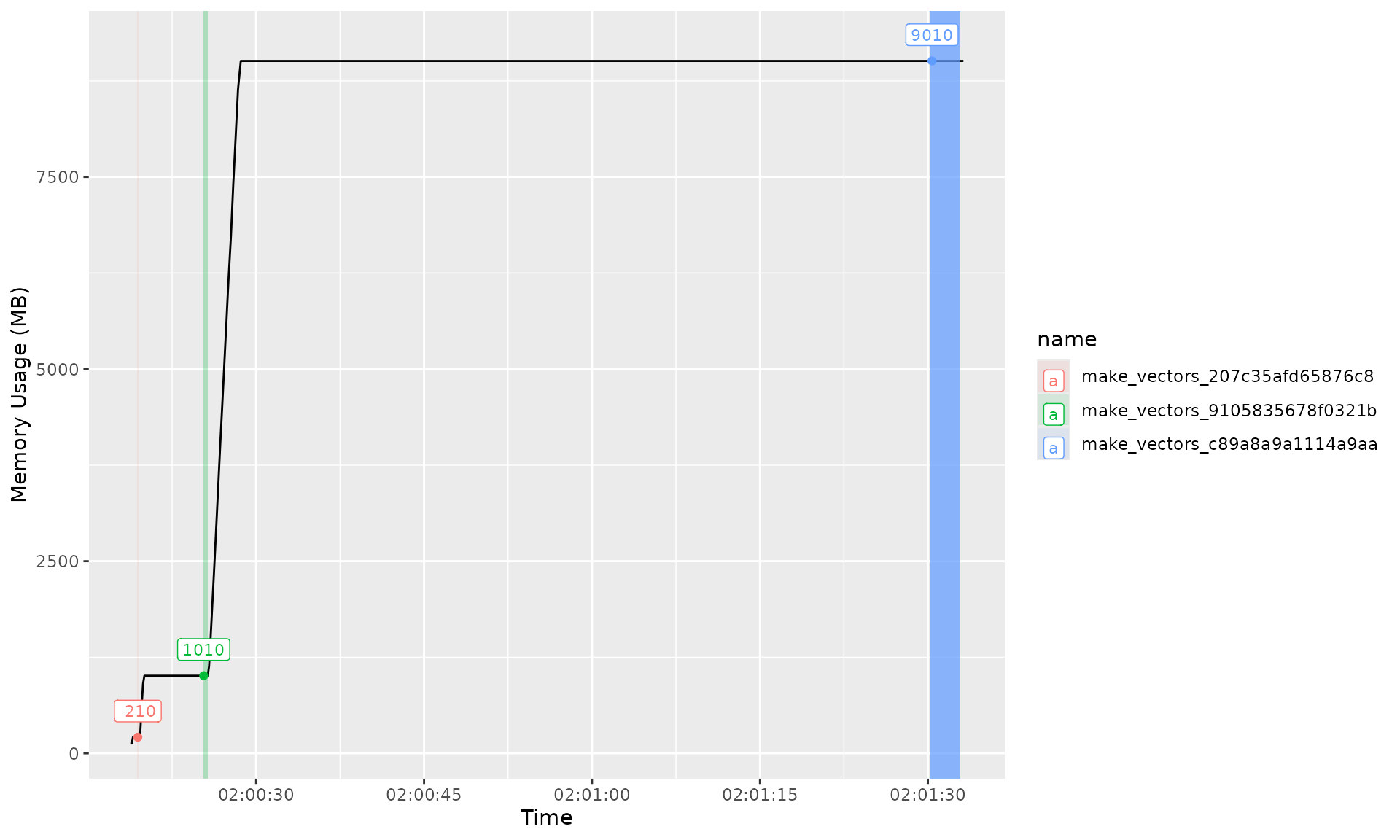
## 3 make_vectors_c89a8a9a1114a9aa  9009582080 2024-05-29 12:01:30          0.895

Finally we can use tarprof::memory_plot to represent the memory usage In the plot below, each colour corresponds to a different target. The coloured band indicates the time that targets thinks the target was running for (although I’m unsure how accurate this is). The labelled point indicates the maximum memory usage for that target. Note that these maximum points correspond to the value of peak_memory in the previous data frame.

tarprof::memory_plot(profile)